An Exemplary Tutorial#
Here is a detailed tutorial to show how to use the executable binary cali or python version pycali by taking the data of Mrk 335 from ASAS-SN and ZTF as an example.
cali#
In the “tests/cali” folder, a jupyter notebook “tests_mrk335.ipynb” is provided. The relevant data “Mrk335_ztf.csv” and “Mrk335_asas.csv” are also provided in the same folder.
The basic steps are similar to the python version detailed below.
pycali#
A jupyter notebook “tests_mrk335.jpynb” and a Python script “tests_mrk335.py” are provided in the folder “tests/” along with the package. The relevant data “Mrk335_ztf.csv” and “Mrk335_asas.csv” are also provided in the same folder.
First download the data of Mrk 335 in a CSV format from ASAS-SN website (https://asas-sn.osu.edu/) and ZTF website (ZTF g band; https://irsa.ipac.caltech.edu/Missions/ztf.html). Suppose the filenames are Mrk335_asas.csv and Mrk335_ztf.csv, respectively.
Load these data and generate a formatted input file for PyCALI.
import numpy as np
import matplotlib.pyplot as plt
import pycali

ztf = pycali.convert_ztf("Mrk335_ztf.csv", rebin=True, errlimit=0.079, zeropoint=3.92e-9, keylabel="")
# rebin:  whether rebin the points within one day
# errlimit: discard these points with errors larger than this limit
# zeropoint is the zero-magnitude flux density
# keylabel is the label added to each dataset. If empty, do nothing.
#
# return a dict, with keys like "ztf_zg", "ztf_zr" etc.
# if keylabel is not empty, the kyes will be keylabel+"ztf_zg" etc.
#

asas = pycali.convert_asassn("Mrk335_asas.csv", rebin=True, errlimit=0.079, diffcamera=False, zeropoint=3.92e-9, keylabel="")
# diffcamera: whether treat different cameras as different datasets
#
# return a dict, with keys like "asas_g", "asas_V" etc.

data = ztf | asassn  # combine the two dicts
# note: if dicts have the same keys, only the data of the key in the last dict are retained.
#       in this case, specify keylabel in the above to make difference.

pycali.format("Mrk335.txt", data)
# write to a file named "Mrk335.txt"

# if only use data in a time range, use
# pycali.format("Mrk335.txt", data, trange=(2458200, 2470000))
Now the input file has been created. Next run PyCALI to do intercalibration.
# setup configurations
cfg = pycali.Config()
cfg.setup(
      fcont="./Mrk335.txt",     # fcont is a string
      nmcmc=10000, ptol=0.1,
      scale_range_low=0.5, scale_range_up=2.0,
      shift_range_low=-1.0, shift_range_up=1.0,
      syserr_range_low=0.0, syserr_range_up=0.2,
      errscale_range_low=0.5, errscale_range_up=2.0,
      sigma_range_low=1.0e-4, sigma_range_up=1.0,
      tau_range_low=1.0, tau_range_up=1.0e4,
      fixed_scale=False, fixed_shift=False,
      fixed_syserr=True, fixed_error_scale=True,
      fixed_codes=[], # fixed_codes is a list to specify the codes that need not to intercalibrate
                      # e.g., [1, 3], will fix 1st and 3rd codes
      fixed_scalecodes=[], # fixed_scalecodes is a list to specify the codes that need to fix scale (to 1)
                      # e.g., [1, 3], will fix scale of 1st and 3rd codes
      flag_norm=True, # whether do normalization before intercalibrating
      )
cfg.print_cfg()

######################################################
# do intercalibration
#
cali = pycali.Cali(cfg)  # create an instance
cali.mcmc()              # do mcmc
cali.get_best_params()   # calculate the best parameters
cali.output()            # print output
cali.recon()             # do reconstruction

# plot results to PyCALI_results.pdf
pycali.plot_results(cfg)

# a simple plot
pycali.simple_plot(cfg)
Now the run ends. The results output in “PyCALI_results.pdf” look like
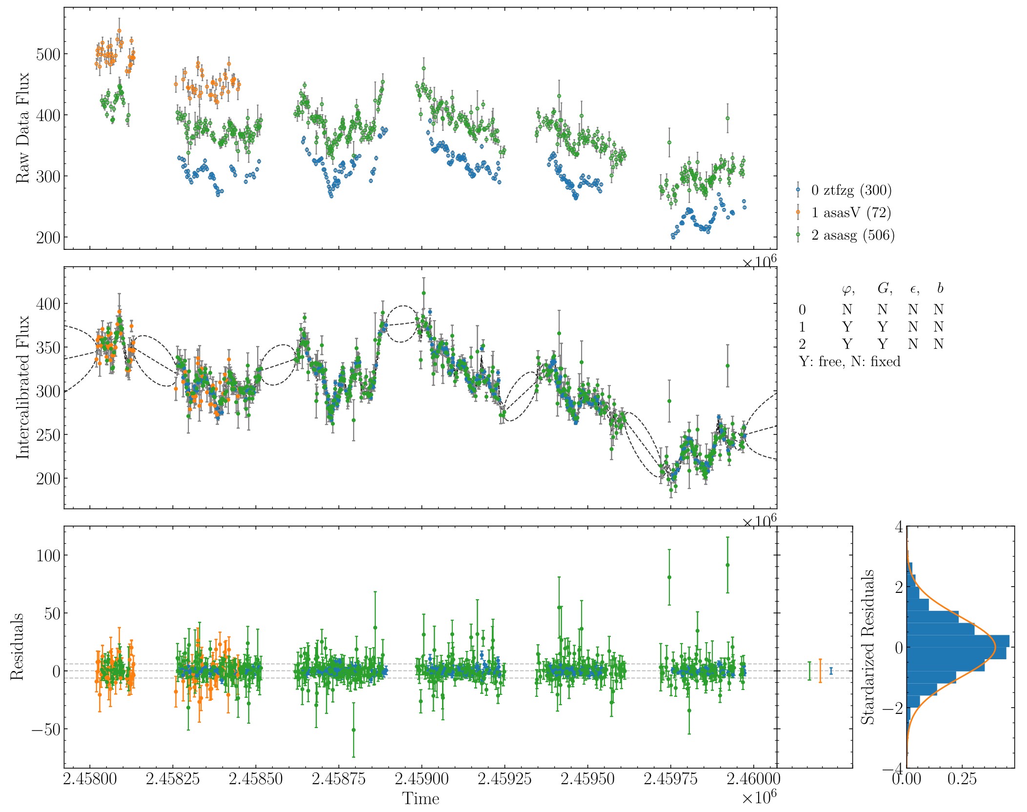
An example of intercalibration for Mrk 335 data from ZTF and ASAS-SN.#
One can also take at look at the intercalibrated data by himself/herself,
data_cali = np.loadtxt("Mrk335.txt_cali", usecols=(0, 1, 2))
code = np.loadtxt("Mrk335.txt_cali", usecols=(3), dtype=str)
fig = plt.figure(figsize=(10, 6))
ax = fig.add_subplot(111)
for c in np.unique(code):
    idx = np.where(code == c)[0]
    ax.errorbar(data_cali[idx, 0],  data_cali[idx, 1], yerr=data_cali[idx, 2], ls='none', marker='o', markersize=3, label=c)

ax.legend()
ax.set_title("Intercalibrated data")
plt.show()
There appears a number of outliers. We can discard these outliers as follows, which are identified once their deviations from the reconstructed light curves using a DRW process are larger than 5sigma.
(Of course, if the intercalibrated results are satisfactory, no need to do the followings.)
pycali.remove_outliers("./Mrk335.txt", dev=5, doplot=True)
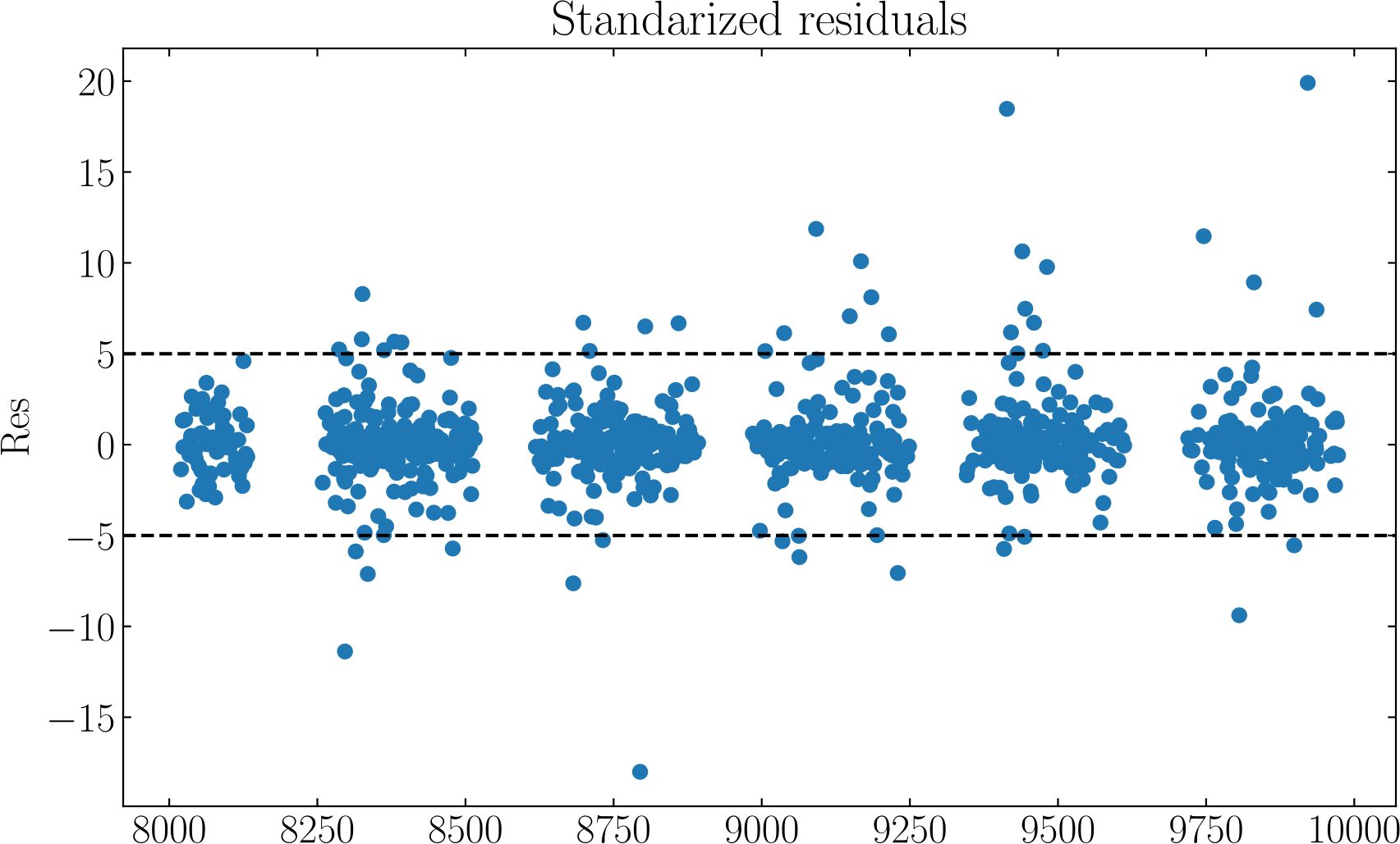
The deviations from the reconstruction (with DRW) and the points beyond the 5sigma deviation are removed.#
This will generate a new data file named Mrk335_new.txt. Now redo the intercalibration on new data.
# setup configurations
cfg = pycali.Config()
cfg.setup(
    fcont="./Mrk335_new.txt",     # fcont is a string
    nmcmc=10000, ptol=0.1,
    scale_range_low=0.5, scale_range_up=2.0,
    shift_range_low=-1.0, shift_range_up=1.0,
    syserr_range_low=0.0, syserr_range_up=0.2,
    errscale_range_low=0.5, errscale_range_up=2.0,
    sigma_range_low=1.0e-4, sigma_range_up=1.0,
    tau_range_low=1.0, tau_range_up=1.0e4,
    fixed_scale=False, fixed_shift=False,
    fixed_syserr=True, fixed_error_scale=True,
    fixed_codes=[], # fixed_codes is a list to specify the codes that need not to intercalibrate
                    # e.g., [1, 3], will fix 1st and 3rd codes
    fixed_scalecodes=[], # fixed_scalecodes is a list to specify the codes that need to fix scale (to 1)
                    # e.g., [1, 3], will fix scale of 1st and 3rd codes
    flag_norm=True, # whether do normalization before intercalibrating
    )
cfg.print_cfg()
######################################################
# do intercalibration
#
cali = pycali.Cali(cfg)  # create an instance
cali.mcmc()              # do mcmc
cali.get_best_params()   # calculate the best parameters
cali.output()            # print output
cali.recon()             # do reconstruction

# plot results to PyCALI_results.pdf
pycali.plot_results(cfg)

# a simple plot
pycali.simple_plot(cfg)
The results output in “PyCALI_results.pdf” now look like
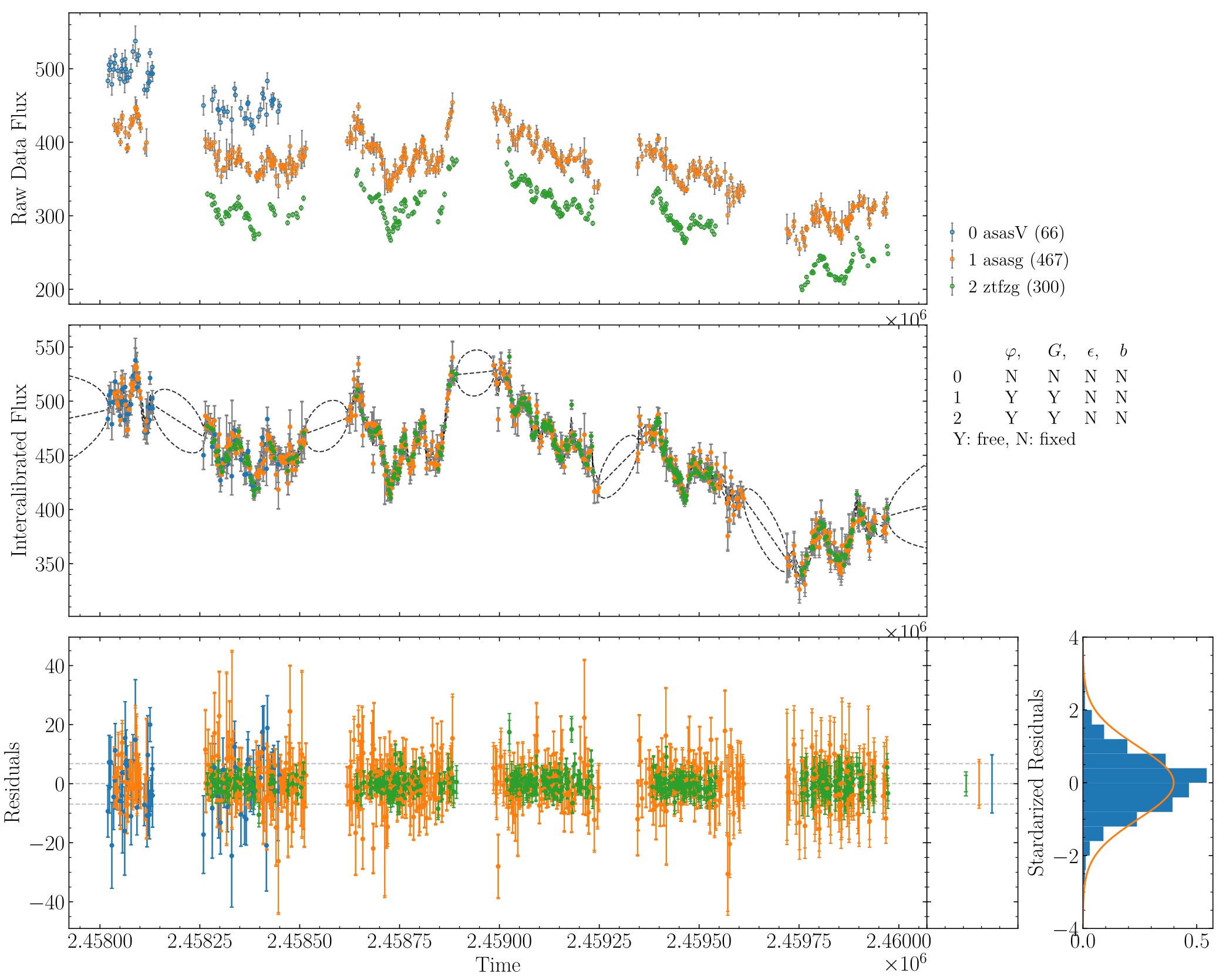
An example of intercalibration for Mrk 335 data from ZTF and ASAS-SN, after remove the outliers.#
Again, one can take a look at the newly intercalibrated data.
data_cali_new = np.loadtxt("Mrk335_new.txt_cali", usecols=(0, 1, 2))
code = np.loadtxt("Mrk335_new.txt_cali", usecols=(3), dtype=str)
fig = plt.figure(figsize=(10, 6))
ax = fig.add_subplot(111)
for c in np.unique(code):
    idx = np.where(code == c)[0]
    ax.errorbar(data_cali_new[idx, 0],  data_cali_new[idx, 1], yerr=data_cali_new[idx, 2], ls='none', marker='o', markersize=3, label=c)

ax.legend()
ax.set_title("Intercalibrated data")
plt.show()