Intercalibration: Methodology and Implementation#
Basic Equations#
By taking \(5100\) A continuum flux densities and H \(\beta\) emission line fluxes as an example, the intercalibration between datasets observed by different telescopes is written
where \(\varphi\) is a multiplicative factor and \(G\) is an additive factor.
Reform the above equations with vectors. We now have \(m\) measurements of a true signal \(y\) by \(k\) different telescopes
where \(n\) are reported measurement noises, \(\epsilon\) are unknown systematic errors, \(b\) is an \(m\times m\) diagnoal matrix for error scale. The above equations stands for continuum flux densities. For emission line fluxes, \(G=0\).
PyCALI uses the damped random walk process to describe the variations and employs a Bayesian framework to determine the best estimates for the parameters by exploring the posterior probability distribution with the diffusive nested sampling algorithm.
Implementation#
In real implementation, the first dataset is set to be the reference with \(\varphi=1\) and \(G=0\).
The input light curve of each dataset is first normalized before being passed to intercalibration (when FlagNorm is set to 1).
The continuum fluxes are normalized as
where \(f_{i, j}\) is the \(j\)-th point of the \(i\)-th continuum dataset and \(C_i\) is the mean, calculated as
where \(N_j\) is the number of points of the \(i\)-th continuum dataset. The emssion line fluxes are normalized as
where \(L_i\) is the mean of the \(i\)-th line dataset, and
This normalization is to enforce that the fluxes are scaled with a same factor as those of continuum. The obtained posterior samples of parameters refer to normalized light curves. That is to say, one needs to mannually do some convertions to obtain the real parameter values. For scale and shift parameters,
For systematic error factor and error scale factors of continuum datasets,
For systematic error factor and error scale factors of line datasets,
Note
The above procedure applies when the option FlagNorm is set to 1 in parameter file or flag_norm=True in python script.
However, when FlagNorm = 0, in the above normalization procedure, the means of each code is set to the same as the reference
code. This is equivalent to no normalization.
Systematic Error and Error Scale#
PyCALI can add systematic errors in quadrature to the data errors as well as scale the data errors, in order to account for the situation that the data errors are not appropriately given (see above). These are controled by the options FixedSyserr and FixedErrorScale, respectively.
In practice, there might be instances that the extent of inappropriate assignment of data errors changes annually or by some periods, meaning that the sysetematic errors to add are not uniform. PyCALI can also handle this situation. Input a flag to each data point to classify the period with a uniform expected systematic error and error scale as follows:
# code1 120
7517.0   1.98   0.08  1
7534.0   2.06   0.08  1
...
7719.0   2.03   0.08  1
7725.0   1.97   0.08  2
7778.0   2.02   0.08  2
# code2 45
7573.0   2.73   0.11  1
7584.0   2.73   0.11  1
...
7644.0   3.45   0.14  2
7661.0   3.26   0.13  2
# code3 33
7509.0   1.92   0.08  1
7530.0   1.97   0.08  1
...
7556.0   2.21   0.09  2
7614.0   2.31   0.09  2
# code4 0
# code5 3
7719.0   2.03   0.08  1
7725.0   1.97   0.08  1
7778.0   2.02   0.08  1
Here, the fourth column is the flag, which should be any integers. PyCALI can automatically recognize this format and read the fourth column as flags. For each code, points with the same flag have the same sysetematic error and error scale. Note that different code still has different sysetematic error and error scale, regardless of the flags.
Outputs#
PyCALI generates a number of outputs to the directory ./data/. If this directory does not exist, PyCALI will create it automatically. Main output files are
xxx_cali
intercalibrated light curve, xxx represents the name of the input data.
xxx_recon.txt
reconstructions to the intercalibrated light curves using the dampled random walk model.
factor.txt
The estimated values of intercalibration parameters, determined from the means and standard deviations of the posterior samples. One may do more sophisticated statitics using the posterior samples. (Note again that these values refer to the light curves normalized by their means, see “Implementation” above).
posterior_sample.txt
posterior samples for intercalibration parameters. The columns are: sigmad and taud (damped random walk model parameters), scale factors, and shift factors; then follow systematic error factors and error scale factors for each light curves (continuum, line1, line2, etc). (Note that the values of these parameters refer to the light curves normalized by their means, see above).
Parameter Values#
The default prior ranges for scale and shift parameters are [0.5-2.0] and [-1.0, 1.0], respectively. This generally work well in most cases. However, there are always exceptions. In the generated file PyCALI_results.pdf, PyCALI plots the posterior distributions of all parameters. When the prior ranges are inappropriate, the distributions will show a cut-off around the lower and/or upper limits. PyCALI add vertical dashed lines to mark the lower and/or upper limits when the parameter hits the limits. In such cases, one needs to adjust the parameter range accordingly. Below shows an example for the scale parameter hiting the limit,
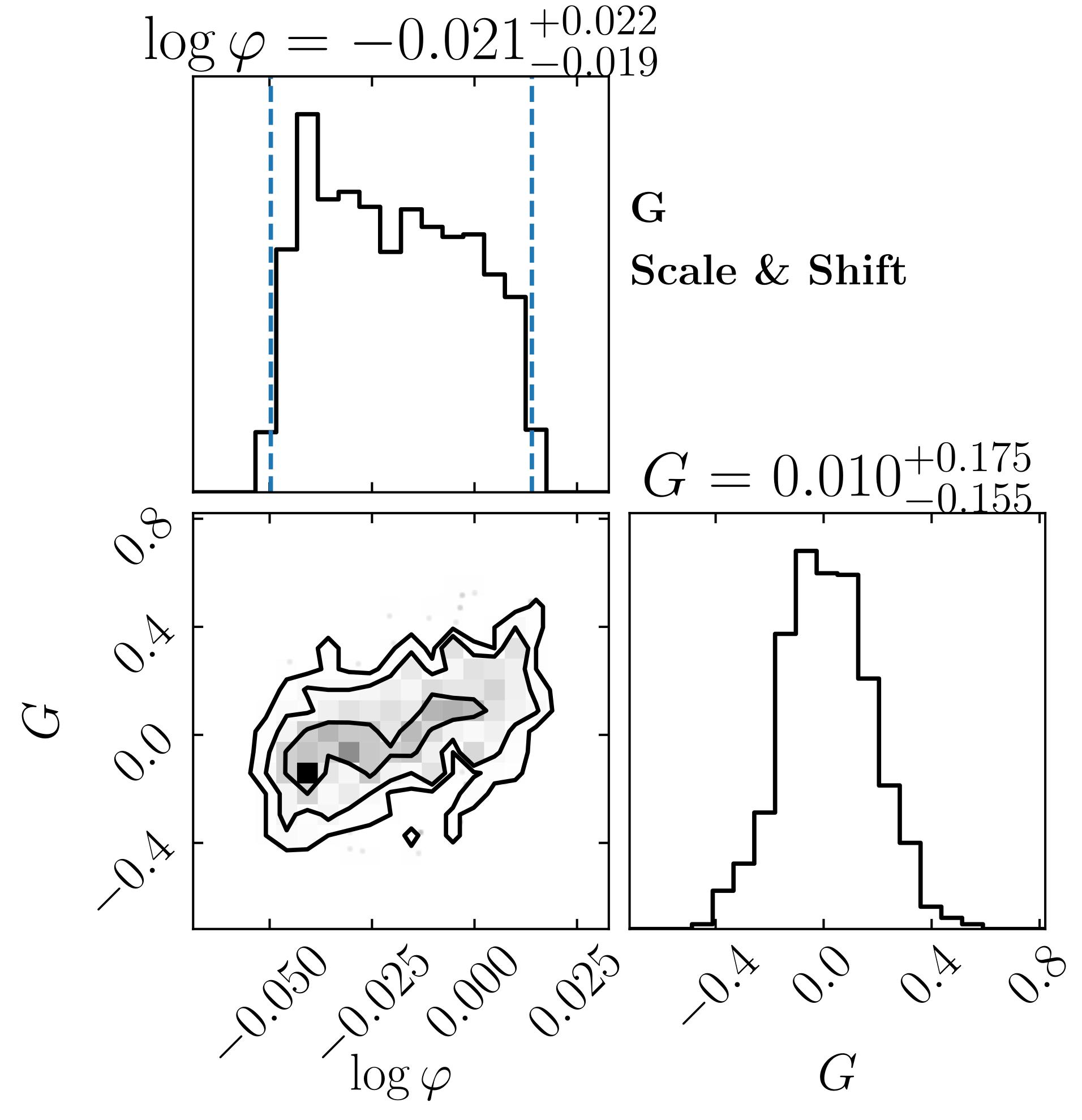
An example where the scale parameter hiting the lower and upper limits (shown by vertical dashed lines). One needs to enlarge the prior prange of the scale parameters accordingly.#
Special Notes#
When a dataset has number of continuum points less than or equal to 2 and no line points, the shift factor is fixed to zero.
The scale and shift factors are highly degenerated. PyCALI implicitly take this degenecy into account when peforming Bayesian sampling.
PyCALI employs the diffusive nested sampling package CDNest (LiyrAstroph/CDNest) to generate posterior samples of intercalibration parameters. The diffusive nested sampling algorithm is developed by Brewer et al. (2011; eggplantbren/DNest4).
Future Improvements#
Presently, PyCALI relies on the damped random walk process to describe light curves. An adaption to flexible variability models is highly worthwhile.